EPID 684
Spatial Epidemiology
4/12/2022
Jon Zelner
[email protected]
epibayes.io
Discuss the qualitative dimensions of residential segregation.
Looking at interacting dimensions of risk using the index of concentration at the extremes (🧊).
Using a hierarchical approach to characterize multi-level patterns of residential segregation.
Smoothing pt. 2 (if ⏰…)
Take a look at the map of county-level segregation here.
Read some of the (short) regional segregation stories.
Pick an area that you are interested in/feel knowledgable about.
Look at patterns of change over time.
How does changing the scale impact what you see/learn from the map?
A function of local and regional dynamics.
Reflects the independent and interacting effects of racial discrimination and economic disparities (1).
Huge regional differences in the nature, causes, and intensity of residential segregation.
Obviously these dynamics stretch the ability of very reductive approaches to show us much that is meaningful.
Capture the impact of extremes
For wealth: \[\text{ICE}_i = \frac{A_i - P_i}{T_i}\]
Where, \(P_i\) = number of poor people in area \(i\), \(A_i\) number of affluent people, and \(T_i\) is total number.
Ranges from -1 to 1
Can be extended to multiple groupings, i.e. number of wealthy individuals in advantaged race/ethnic group - number of poor individuals in disadvantaged race/ethnic group.
What does the ICE let us learn in the Feldman (2) piece that we wouldn’t have otherwise?
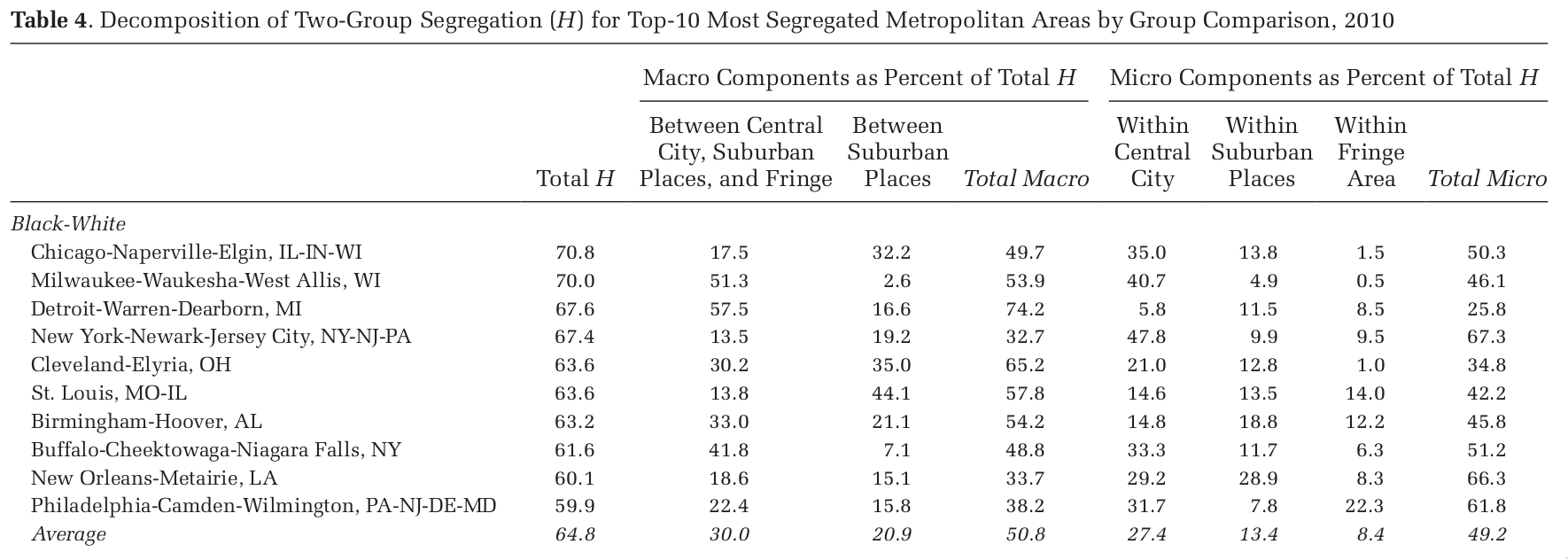
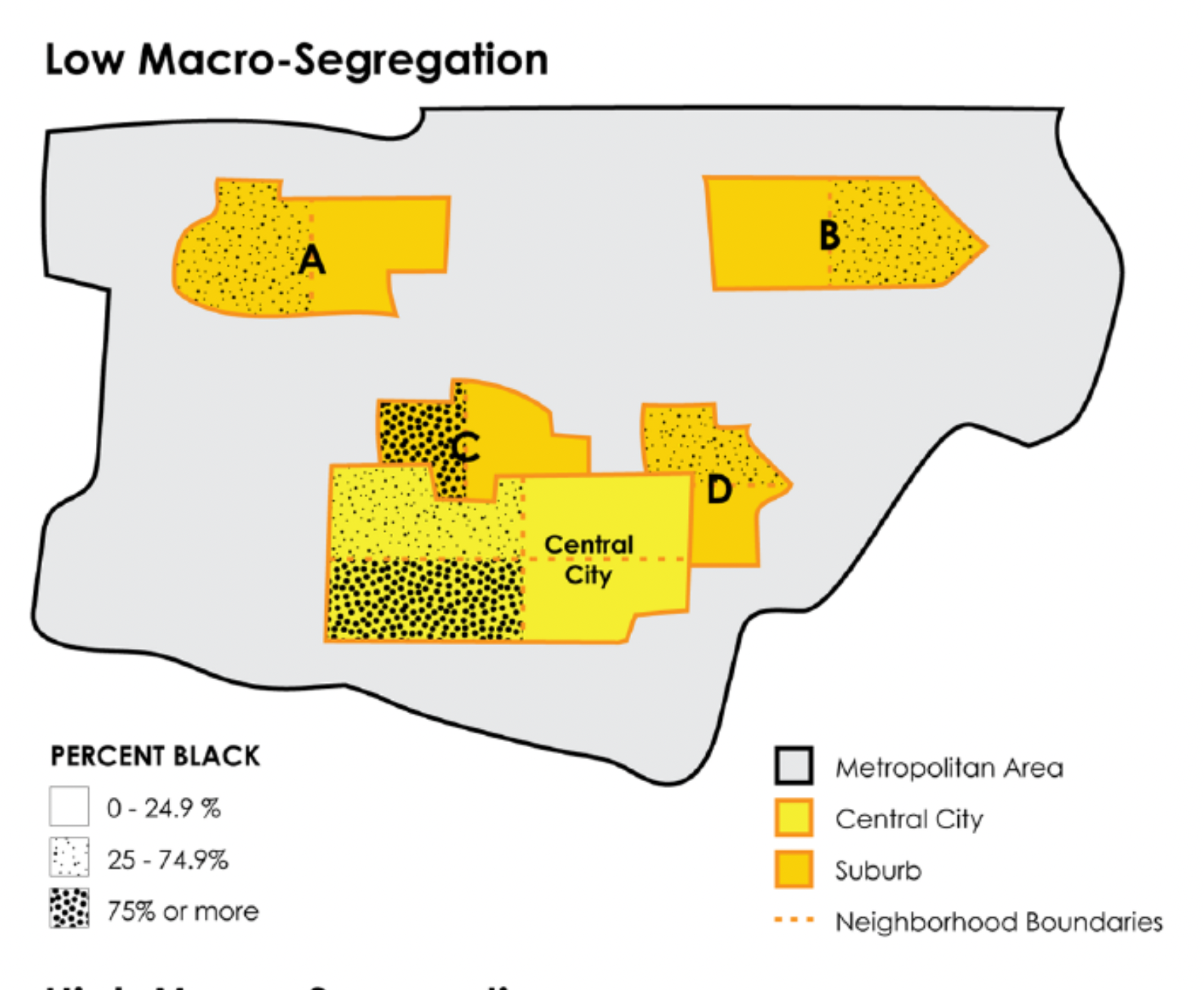
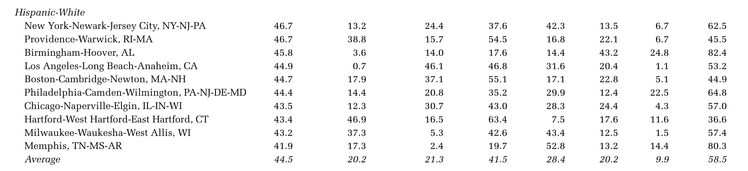
An example where segregation is primarily explained by within-unit variation. (from Lichter & Parisi (3))
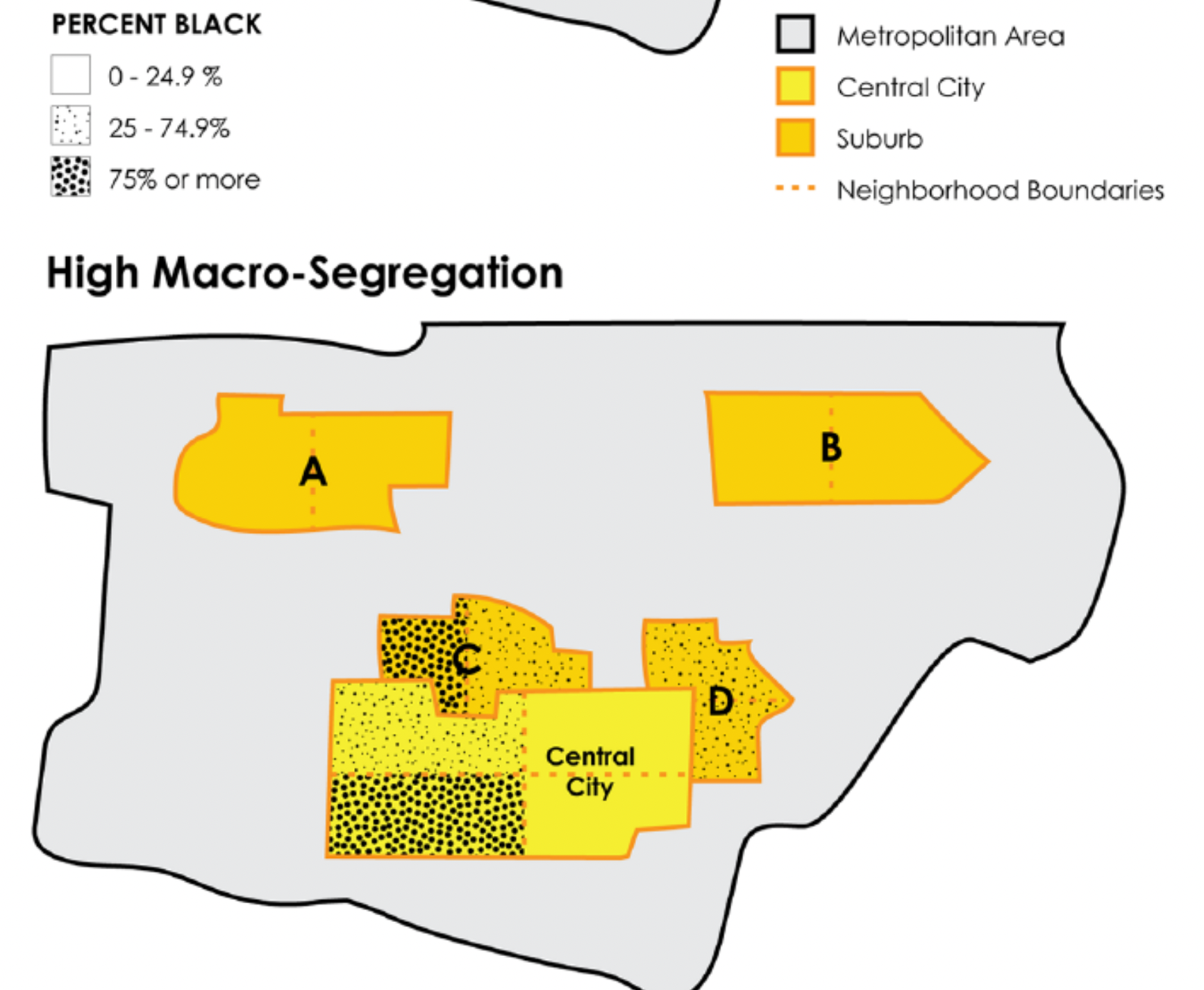
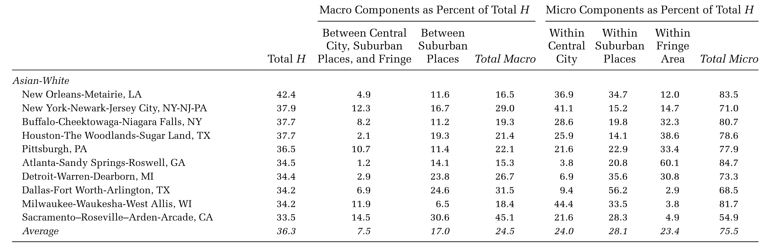
A pattern of segregation dominated by between-unit variation (3)
Dissimilarity & Isolation only characterize variation within the lowest levels observed.
Moran’s I includes information on proximity or adjacency but is also only focused on lowest-level relationships.
Lichter and Parisi (3) use the Thiel index - an entropy-based measure - to characterize the overall intensity and scale of residential segregation.
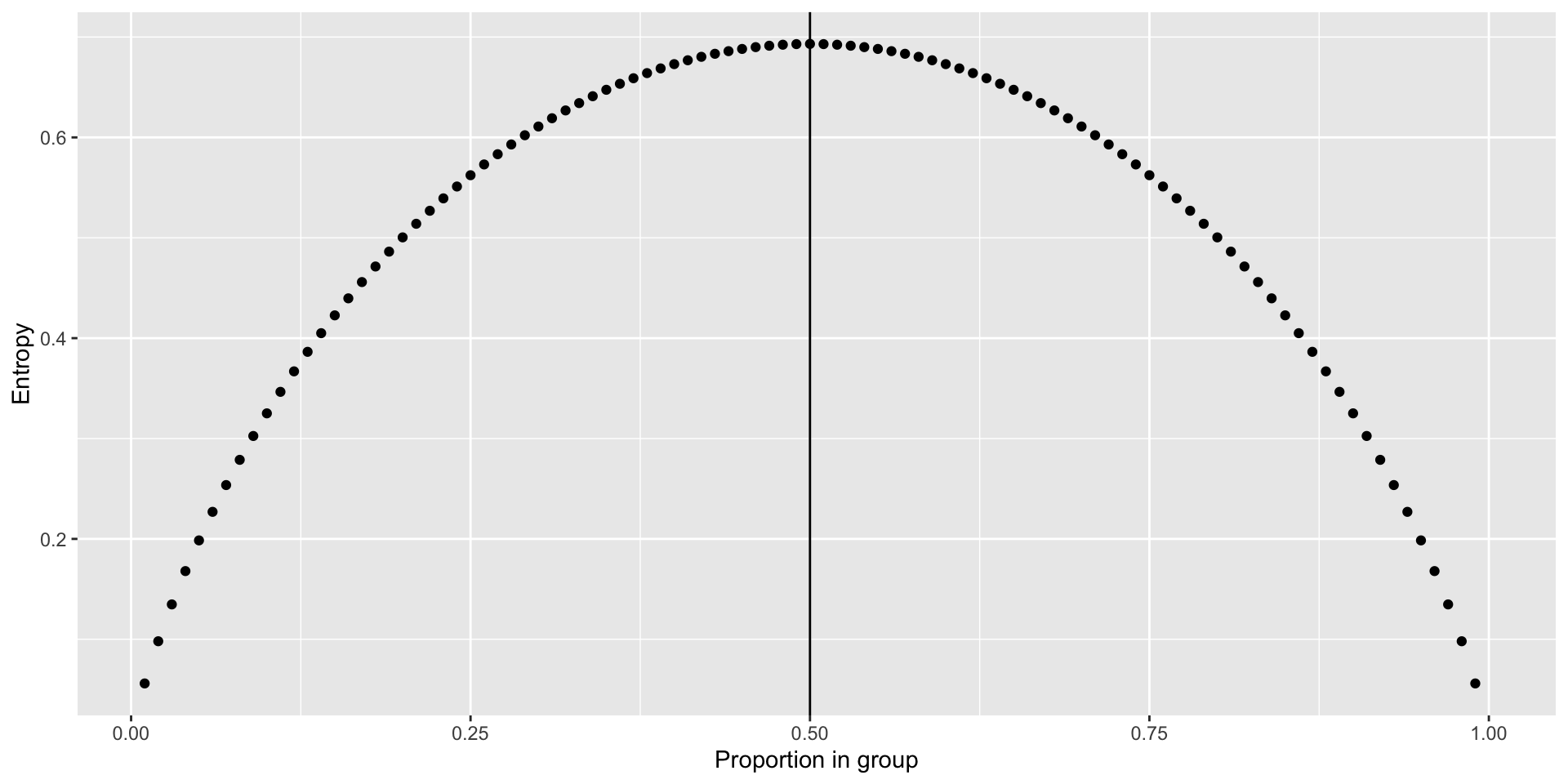
Entropy (\(E\)) is a measure of uncertainty
Maximum value \(\to\) Maximum Uncertainty
Minimum value Minimum Uncertainty
For two groups: \[E = p \frac{1}{p} + (1-p)\frac{1}{1-p}\]
Not limited to binary comparisons
A weighted average of differences in entropy between different levels.
If \(H=0\), the entropy within all lower-level units is equivalent to the population-level entropy.
In other words, all variation is within-unit.
If \(H=1\), the total amount of population-level entropy is explained by between-unit variation.
\[ H_{B \in M} = \frac{1}{N_M E_M} \sum_{b=1}^{B}N_B(E_M-E_b) \]
Where:
\(H\) is a sum over neighborhood-level differences from the population entropy.
To see what the contribution of a given level is to the overall H, we just look at the sum over all smallest-level units in the one we care about.
This lets us ask what proportion of the total \(H\) in an area can be attributed to variation within and between different types of units within a metro area.
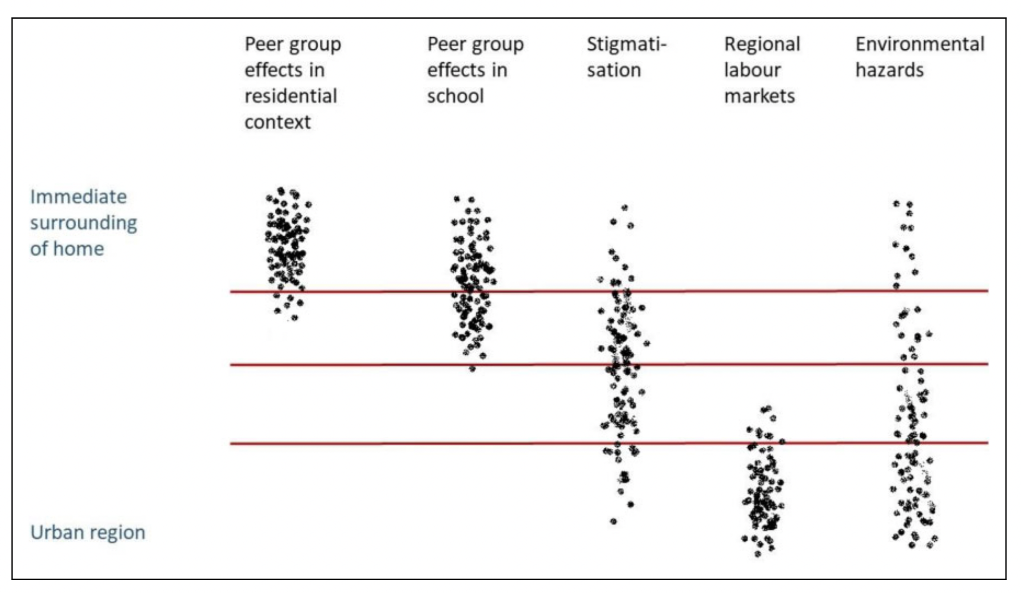
Can theses approaches help us pick more relevant scales of analysis? (Figure from (4))
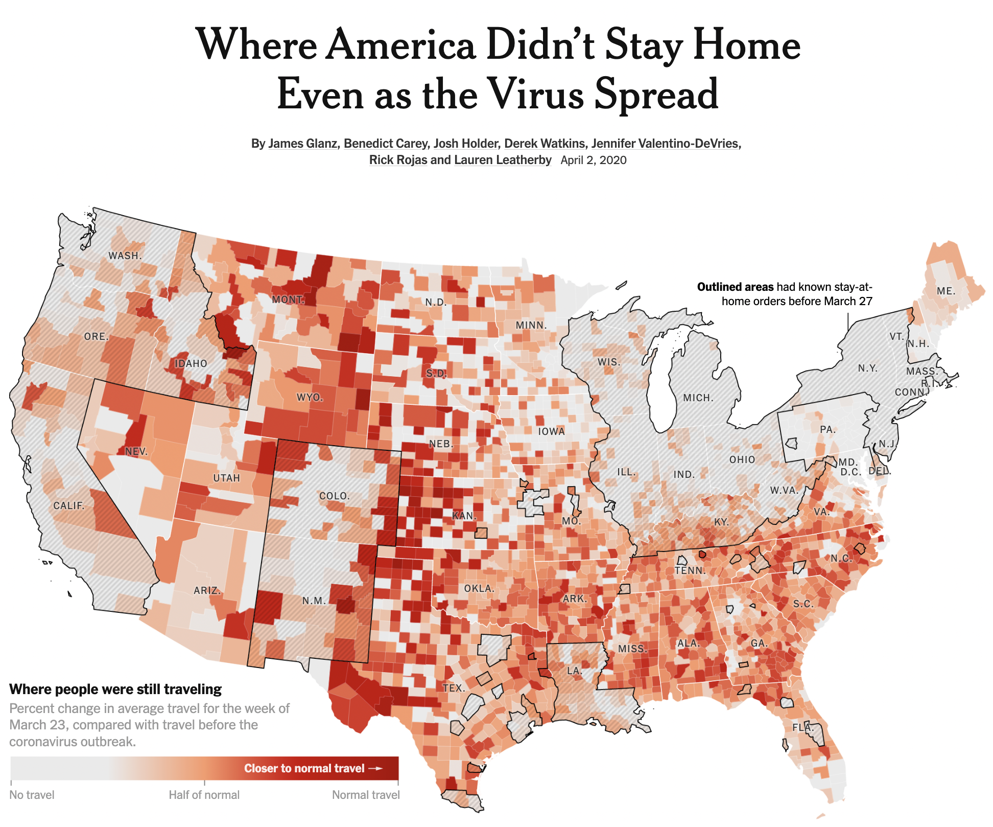
Relating mobility to COVID-19 spread in the early days of the pandemic (5)